Tutorials
This page contains two tutorials:
Read and explore OCT data
This tutorial shows how to:
Load OCT files into MATLAB
Visualize loaded data (fundus image, OCT slices, segmentation…)
Generate a visual report
The source code of this tutorial can be found in the tutorials folder or here.
0. Understand your data
The first step is to understand your images in terms of:
Device and file format: there are many different devices and file formats and not all of them are equally easy to read and have the same information.
Acquisition protocol: OCT images are composed of one or more 2D images (aka slices or B-scans). It is crucial to know the area covered by these B-scans (macula, optic disk, wide), as well as their geometrical arrangement (horizontal, circular).
Understanding the above will help troubleshoots problems.
RETIMAT can only read vol, e2e, fda, img files. If your files are different, you can try the following Python packages:
1. Load the images
Images are loaded into MATLAB by means of dedicated read functions.
For instance, a Heidelberg vol file can be read as:
[header, seg, bscan, fundus] = read_vol(file)
This function returns four arguments:
header: struct with metadata (image sdimensions, lateraliry, …)seg: struct with retinal layer segmentationbscan: a 3D image with B-scansfundus: a 2D image with a fundus image
Other file formats can be read similarly:
[header, seg, bscan, fundus] = read_e2e(file)
A single E2E file can contain more than one OCT volumes (usually two: one per eye).
For this reason, the returned objects are cell lists each related to a single OCT volume.
Topcon fda files contain metadata, OCT, segmentation and a color fundus image. To read them:
[header, seg, bscan, fundus] = read_fda(file)
Cirrus img files only contain 1 OCT volume and no segmentation or metadata.
The read_img function reads the B-scans and tries to infer the metadata from image size and file name.
[header, bscan] = read_img(file)
The fundus image acquired along with the img is stored in a separated bin file that can be read by:
fundus = read_bin(file)
2. Explore metadata
After reading a file, it is a good idea to look into the metadata stored in the header to check that everything looks good.
We can do that with the following command:
disp(header)
Header structure is an attempt at harmonizing data from different scanners.
Fields should be equivalent across scanners. However, due to the difficulty of fully reading propietary file formats, not all the fields will be present for every format.
We can also check which segmented layer boundaries are present in the file:
boundaries = fields(seg);
disp(boundaries')
3. Visualize the images
Quality assurance is a key step in any image analysis pipeline. In OCT, poor contrast, artifacts, and segmentation errors are not uncommon. Therefore, it is crucial to inspect the data to detect those problems.
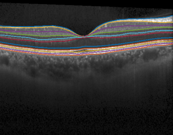
Here we plot the middle B-scan with its segmentation:
f = figure;
idx_bscan = 13;
imshow(bscan(:,:,idx_bscan)); hold on;
for j=1:length(boundaries)
    plot(seg.(boundaries{j})(idx_bscan, :))
end
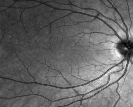
Often a fundus image is acquired alongside the OCT volume. Depending on the scanner this image is different:
Heidelberg: a graysacle image stored in
vol,e2efiles.Cirrus: a grayscale image stored in a separated
binfileTopcon: an RGB color image stored inside
fdafiles.
To visualize the fundus image we can just:
f = figure;
imagesc(fundus); colormap(gray); axis("off");
4. Generate a report
Doing all the previous steps separately is not always convenient.
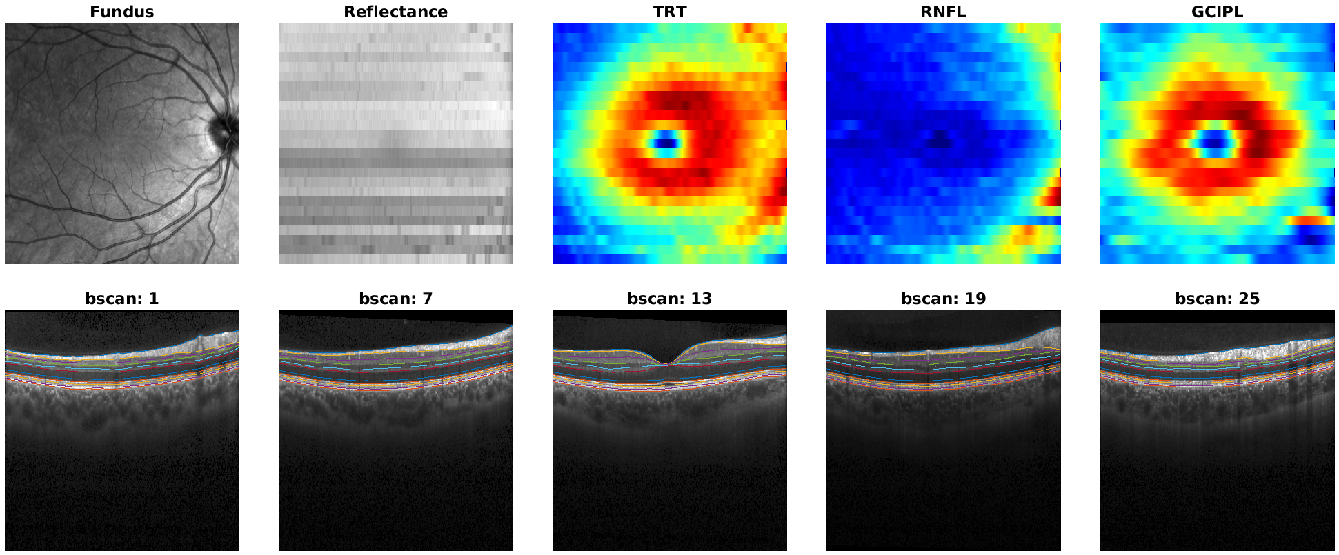
To simplify data inspection, we can automatically create a summary report using the generate_report() function.
The function allows us to pass fundus,bscan and segmentation data and builds a tiled plot that can be stored in memory.
A full report includes:
Fundus image
Reflectance map: a 2D map obtained by averaging A-scan intensities in depth. Useful to detect noisy B-scans and shades.
Thickness maps: 2D maps generated by computing layer thicknesses from segmentation data. Useful to detect segmentation errors or lessions.
B-scans: several slices with overlapping segmentation.
As an example, let’s generate a full report for the loaded image.
As arguments we need to provide image data and the layers for which we want to plot thickness maps
layers = {'TRT','RNFL','GCIPL'};
generate_report(bscan, seg, fundus, layers);
Finally, to store it as a png withoug opening a window:
generate_report(bscan, seg, fundus, layers, 'file_name', 'report.png', 'visible', 'off');
Feature extraction
This tutorial shows how to build a feature extraction pipeline step by step
0. Preliminaries
The computation of retinal features requires the segmentation or retinal layer boundaries.
Here, there are two possiblities:
The images were already segmented and the segmentation is stored in vol, e2e, or fda files
We have raw images without segmentation
We can check that by reading the images and trying to visualize the segmentation as in the previous tutorial.
In the segmentation is not available, we recommend using OCT Explorer software to do so. OCT Explorer allows you to load your images and save the segmentation as an xml file that can be read by RETIMAT.
After segmentation, we need to decide which features we want to compute. There are four categories of features:
Thickness: average thickness values over predefined macular sectors.
Foveal pit morphology: geometrical features of the foveal pit morphology (slope, radius, …).
Reflectance: features related with image intensity.
Texture analysis: features that measure statistical properties of the thickness surface.
Each feature type requires a different set of processing steps. In the next steps basic thickness feature extraction is described. The source code of is available. If you want to extract non-thickness features please check the other tutorials.
1. Load the files
This step parses the information inside the file and computes the X, Y coordinates of each A-scan.
To analyse retinal thickness we only need the header and the segmentation data.
[header, seg, ~, ~] = read_vol(file, 'get_coordinates');

X = header.X_oct;
Y = header.Y_oct;
2. Preprocessing
We can now compute thicknesses as the difference between segmented boundaries.
We need to specify the layers to analyse as input.
Thickness values are by defaul in pixels, but can be computed in micrometers if we pass the axial resolution (scale_z) to the function.
The output are stored in the struct Thickness with a field for every layer.
layers = {'TRT', 'GCIPL'};
Thickness = compute_thickness(seg, layers, header.scale_z);

TRT = Thickness.TRT;
GCIPL = Thickness.GCIPL;
To compute averaged sector thicknesses it is convenient to have regular spatial sampling (i.e., same sampling distribution across the macula). To achieve that we can transform our original A-Scan coordinates to a regular grid by using interpolation.
[X_new, Y_new, TRT_new] = resample_map(X, Y, TRT, 'regular', 'max_d', 3, 'n_point', 100);
[X_new, Y_new, GCIPL_new] = resample_map(X, Y, GCIPL, 'regular', 'max_d', 3, 'n_point', 100);
3. Foveal location
Often, acquired images may not be correctly centered at the foveal pit (due to fixation errors). This can result in erroneous measurement and must be corrected. To do this we need to:
Locate the actual foveal center automatically
Set
X,Ycoordinate origin to the foveal center
[x_fovea, y_fovea] = find_fovea(X, Y, TRT);

X = X - x_fovea;
Y = Y - y_fovea;
4. Sectorize thickness
Often we are interested in average measures of the thickness maps of above.
For instance, to compute ETDRS sectorized we just need to:
[TRT_etdrs, Sect_etdrs]  = sectorize_map(X_new, Y_new, TRT_new, 'mean', 'etdrs');
[GCIPL_etdrs, Sect_etdrs] = sectorize_map(X_new, Y_new, GCIPL_new, 'mean', 'etdrs');
This returns the averaged numeric values: TRT_etdrs and a Sect_etdrs struct.
ETDRS sectors are: central, inner nasal, inner superior, inner temporal, inner inferior, outer nasal, outer superior, outer temporal and outer inferior
etdrs_vars = {'C', 'IN', 'IS', 'IT', 'II', 'ON', 'OS', 'OT', 'OI'};
T = cell2table([layers' num2cell([TRT_etdrs; GCIPL_etdrs])], 'VariableNames',[{'layer'}, etdrs_vars])
We can also use more advanced sectorizations
Sectors.type    = 'wedge';
Sectors.radius  = linspace(0, 3, 10);
Sectors.theta_0 = 0;
Sectors.n_angle = 20;
Sectors.n_sect  = Sectors.n_angle * (length(Sectors.radius) - 1);

[TRT_wedge, Sect_wedge]  = sectorize_map(X_new, Y_new, TRT_new, 'mean', Sectors);
[GCIPL_etdrs, Sect_wedge] = sectorize_map(X_new, Y_new, GCIPL_new, 'mean', Sectors);
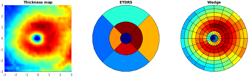
5. Visualize results
We can visualize custom sectorizations by using plot_sectors()
f = figure('Position', [0 0 1200 400]);

subplot(131);
surf(X_new, Y_new, TRT_new, 'EdgeColor', 'none'); view(0,90);
axis equal;
title('Thickness map')

subplot(132);
plot_sectors(TRT_etdrs, Sect_etdrs); title('ETDRS');

subplot(133);
plot_sectors(TRT_wedge, Sect_wedge); title('Wedge');

colormap("jet")